Mathematics & Technology

The real mathematics, statistics, algorithms and physics behind Lotto Simulator — taken from the code that runs in the app.

Open Lotto Simulator

How to read this page

Every formula below is copied from the implementation, not from a brochure. Where a component is a deterministic rule or a heuristic rather than a formula, we describe the algorithm exactly as it runs and do not invent mathematics for it.

Lotto Simulator is an analytical, educational and simulation environment. It generates combinations with sixteen methods, reviews them in a Mathematical Court of twelve jurors, six defence counsel and a Supreme Judge, tests real draw histories for fairness, analyses calendar coincidences and replays a physical 3D lottery drum. None of this changes the probability of any number in an official draw — section 8 explains why, with the numbers.

Notation used throughout

where

$N$: size of the main number pool (for example 50 in Eurojackpot)
$k$: how many main numbers are drawn and played (5 in Eurojackpot)
$B,\; b$: size of the separate bonus pool and how many bonus numbers are played (12 and 2 in Eurojackpot)
$D$: number of past draws in the selected analysis window
$c_n$: how many times number $n$ appeared among the main numbers of those $D$ draws
$t = 0, 1, \dots$: draw index, newest first: $t = 0$ is the latest draw
$\binom{n}{r}$: binomial coefficient, the number of ways to choose $r$ items out of $n$

1. System architecture

One application, one code base: the same web app runs in desktop and mobile browsers and, unchanged, inside the iOS and Android apps (Capacitor WebView). Heavy and paid computation runs on the server; everything the user sees is rendered on the device.

Device (web, iOS, Android)Interface, ticket and working sets, the four FREE generator methods, frequency charts, χ² test, calendar maths, 3D drum. Pure random and the 3D drum take their randomness from the Web Crypto API.
Edge functions (TypeScript, Deno)The twelve PRO generator methods, all nineteen Court models, the twelve jurors, six counsel, the Supreme Judge, wheel designs, the prediction ledger. The Court runs on seeded, reproducible random streams.
Database (PostgreSQL)Official draw results with their rule version, payout tables, accounts and entitlements, the append-only prediction ledger and its evaluation.
Data pipelineScheduled jobs collect official results, validate every draw against the rules of its era and publish the current-rules data set.

Who computes what

In the browser: the FREE methods (Hot numbers, Combined, Segment coverage, Pure random) and all descriptive statistics. The public build physically removes the PRO implementations from the client: their functions are replaced by stubs, so a PRO result can only come from the server.
On the server: every PRO method, the whole Mathematical Court and the Supreme Judge. A request carries the lottery, the method, the number of rows (1–50) and the analysis window; the server loads the draws itself, so the client cannot feed it invented history.
Fail-closed rule: a server model needs at least 5 draws in the selected analysis window. With fewer it refuses with an explicit "insufficient history" answer instead of producing rows from nothing.

Reproducible Court computation

Every juror, counsel and model inside the Court runs on its own pseudo-random stream whose seed is a hash of the algorithm version, the persona, the lottery, the complete draw history and the target draw date. The same data therefore always produces the same verdict, and any change to the history changes every stream.

h_1 = \operatorname{FNV1a}(H;\ h_0), \quad h_2 = \operatorname{FNV1a}(g \,\|\, d;\ h_1), \quad s = \operatorname{FNV1a}(v \,\|\, \kappa;\ h_2), \qquad u_i = \operatorname{mulberry32}(s)_i \in [0,1)

Seed of a Court computation and the stream of uniform numbers drawn from it.

where

$v$: algorithm version of the Court engine
$\kappa$: persona or model key, for example a juror's identifier
$H$: every draw of the window, main and bonus numbers in order
$g,\; d$: lottery identifier and target draw date
$h_0$: the FNV-1a offset basis; $\operatorname{FNV1a}(x;\,h)$ hashes the text $x$ starting from the state $h$
$u_i$: the $i$ -th uniform random number of the stream

Persistence and provenance

Every combination carries a provenance record: its source (generator method, juror, jury consensus, wheel, 3D draw, Supreme Judge, manual entry), the numbers it started with and an append-only event log of reviews, proposals, counsel positions, verdicts, decisions and transformations (at most 200 events). A record is accepted only if replaying its transformations on the initial numbers reproduces the row exactly; otherwise the row is shown as having an unavailable source.

R_m = \bigl(\tau_m \circ \cdots \circ \tau_2 \circ \tau_1\bigr)(R_0)

Provenance check: the current row R_m must equal the initial row R_0 with every recorded replacement τ₁ … τₘ applied in order.

Lineage: when a row is edited by hand, a new record is created whose parent is the previous one (up to four earlier records are kept), so the history before the manual change remains visible.
Prediction ledger: every recommendation (a generated row, a juror's replacement, a counsel's position, a verdict) is written to a ledger before the target draw and evaluated automatically after the official result.

2. Main generator: sixteen methods

The generator offers sixteen selections. Four FREE methods run in the browser; twelve PRO methods run on the server. All of them pick $k$ distinct numbers from $1..N$ plus the bonus numbers of the lottery; they differ only in how numbers are weighted or constructed.

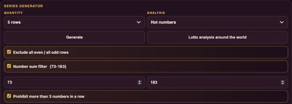
The Series generator with the quantity, the analysis method and the three default filters — The generator panel: method selector and the default filters

Shared building blocks

Weighted methods assign a weight $w_n \ge 0$ to every number and then draw sequentially without replacement: each pick removes the number and renormalises the remaining weights.

P\bigl(x_j = n \mid x_1,\dots,x_{j-1}\bigr) = \frac{w_n}{\displaystyle\sum_{m \notin \{x_1,\dots,x_{j-1}\}} w_m}

Sequential weighted sampling without replacement, used by every weight-based method.

where

$x_j$: the $j$ -th number picked for the row, $j = 1,\dots,k$
$w_n$: the method's weight of number $n$

Randomness: in the browser, Pure random and the uniqueness step use the Web Crypto API, while Hot numbers, Combined and Segment coverage use the browser's standard generator (Math.random). On the server the methods draw from cryptographic randomness, except the Physical model (standard generator) and the Chaos seed, which mixes cryptographic randomness with a high-resolution timer. In the browser an unbiased integer in $0..M-1$ is obtained by rejection sampling, so no residue is favoured:

r = x \bmod M, \qquad x \sim \mathcal{U}\{0,\dots,2^{32}-1\} \ \bigm|\ x < 2^{32} - \bigl(2^{32} \bmod M\bigr)

Rejection sampling: a 32-bit cryptographic value x is redrawn until it falls below the largest multiple of M, then reduced modulo M.

Bonus numbers

Bonus numbers (Eurojackpot 2 of 12, EuroMillions 2 of 12, Powerball 1 of 26, Mega Ball 1 of 24, Viking number 1 of 5, Powerball AU 1 of 20) are drawn from their own pool, independently of the main numbers. Lotto, SuperEnalotto and Lotto Max have no bonus number for the player: their extra ball is drawn by the operator from the main drum.

w'_j = \begin{cases} c'_j + 0.05 & \mu = \mathtt{freq} \\ 1 & \mu \in \{\mathtt{rnd}, \mathtt{phys}, \mathtt{chaos}, \mathtt{world}\} \\ c'_j + 2 & \mu \notin \{\mathtt{freq}, \mathtt{rnd}, \mathtt{phys}, \mathtt{chaos}, \mathtt{world}\} \end{cases}

Weight w′ⱼ of bonus number j with bonus count c′ⱼ for method μ: freq = Hot numbers; rnd, phys, chaos, world = Pure random, Physical model, Chaos, World methods; all other methods use c′ⱼ + 2. With fewer than 5 draws every method uses uniform weights.

FREE filters and uniqueness

Rows produced in the browser pass three filters that are switched on by default: not all numbers even or all odd; the sum inside a range; no run of more than three consecutive numbers. A rejected row is replaced by a uniformly random row that passes the filters (its bonus numbers are drawn with the Bayes weights $c'_j + 2$ ).

\bar S = \frac{k(N+1)}{2}, \qquad \Delta = \max\!\bigl(18,\ \operatorname{round}(0.22\,Nk)\bigr), \qquad S \in \bigl[\max(k, \operatorname{round}(\bar S - \Delta)),\ \min(kN, \operatorname{round}(\bar S + \Delta))\bigr]

Default sum range. Eurojackpot: S̄ = 127.5, Δ = 55, range 73–183.

To avoid handing out the same combination twice on the same device, each FREE row is identified by the lexicographic rank of its main numbers among all $\binom{N}{k}$ combinations and compared with the last 20 000 rows issued for that lottery; a repeated rank is altered by random swaps, and as a last resort the next unused rank is taken from a random affine permutation of all ranks. A row altered in this way is not checked against the filters again.

\operatorname{rank}(x_1 < \dots < x_k) = \sum_{i=1}^{k} \ \sum_{v = x_{i-1}+1}^{x_i - 1} \binom{N - v}{k - i}, \quad x_0 = 0; \qquad \rho_j = (a\,j + b) \bmod \binom{N}{k},\ \gcd\!\bigl(a, \tbinom{N}{k}\bigr) = 1

Lexicographic rank of a combination and the full-period affine walk over all ranks.

FREE and PRO execution paths

Path	Methods	Where it runs	Rows per run	History
FREE	Hot numbers, Combined, Segment coverage, Pure random	browser	up to 5 (up to 50 for PRO users)	the FREE window of recent draws
PRO	the twelve other methods	server	up to 50	the selected analysis window, at least 5 draws

Hot numbers

FREEIn the browser

Purpose: favour the numbers that appeared most often in the analysis window.

w_n = c_n + 0.05

Weight of number n; with fewer than 5 draws all weights equal 1.

Advanced details

Combined

FREEIn the browser

Purpose: mix hot, medium and cold numbers in a fixed proportion.

Numbers are sorted by $c_n$ (ties keep the smaller number first) and split into thirds of size $\lceil N/3 \rceil$ : hot, middle, cold. Row $i$ takes uniform picks from each third:

h = \max\!\bigl(1, \operatorname{round}(0.4k)\bigr), \qquad a = \Bigl\lfloor \frac{k-h}{2} \Bigr\rfloor, \qquad (m_i, c_i) = \begin{cases} (a,\ k-h-a) & i \equiv 1 \pmod 2 \\ (k-h-a,\ a) & i \equiv 0 \pmod 2 \end{cases}

Row i takes h hot, mᵢ middle and cᵢ cold numbers; odd and even rows swap the middle and cold shares.

Advanced details

Segment coverage

FREEIn the browser

Purpose: spread a row evenly across the number range.

s = \Bigl\lfloor \frac{N}{k} \Bigr\rfloor, \qquad x_p \sim \mathcal{U}\{\,p\,s + 1, \dots, (p+1)\,s\,\}\ \ (p < k-1), \qquad x_{k-1} \sim \mathcal{U}\{(k-1)\,s + 1, \dots, N\}

One uniform number from each of k consecutive segments; the last segment takes the remainder.

Advanced details

Pure random

FREEIn the browser

Purpose: the honest baseline — every number equally likely.

P(x_1,\dots,x_k) = \binom{N}{k}^{-1}

A cryptographic Fisher–Yates shuffle gives every combination the same probability before filtering.

Advanced details

Wheel matrix

PROServer

Purpose: build several rows that together cover as many pairs of a small number pool as possible — a greedy covering design.

The pool has $\min(N, k+5)$ numbers taken alternately from the hot, cold and middle thirds. All $\binom{|P|}{k}$ combinations of the pool are candidates (above 40 000 a random sample is used); each step adds the candidate with the best score and marks its pairs as covered:

\operatorname{score}(R) = 100\,\Bigl|\tbinom{R}{2} \setminus \mathcal C\Bigr| \;-\; 6 \sum_{n \in R} u_n \;-\; 2\,\bigl[\max R - \min R < \lfloor \max P / 3 \rfloor\bigr]

Greedy pair-coverage score; ties are broken uniformly at random.

Advanced details

where

$\tbinom{R}{2},\ \mathcal C$: the pairs of the candidate row $R$ and the pairs already covered by the chosen rows
$u_n$: how many already chosen rows contain number $n$
$[\,\cdot\,]$: equals 1 if the condition holds, otherwise 0

World hot and World combined

PROServer

Purpose: transfer the frequency profile of all nine supported lotteries onto the current one.

Each drawn number $x$ of every lottery $g$ is mapped to its relative position $q = (x-1)/(N_g - 1)$ and spread with a narrow Gaussian kernel onto the numbers of the current lottery; every lottery gets the same weight per draw, and the current lottery's own frequency is added once more on top:

S(n) = 10^{-4} + \sum_{g} \frac{1}{D_g} \sum_{x \in X_g} \exp\!\Bigl(-\frac{(q_n - q_x)^2}{2\sigma^2}\Bigr) + 1.8\,\frac{c_n}{D}, \qquad q_n = \frac{n-1}{N-1},\ \ \sigma = 0.035

World score of number n; X_g are all main numbers drawn in lottery g (up to 400 recent current-rules draws, D_g draws).

Advanced details

World hot: $k$ uniform picks from the $\max(3k, 12)$ numbers with the highest score.
World combined: $\lceil 0.45k \rceil$ from the top third, $\max(1, \lfloor 0.2k \rfloor)$ from the bottom third, the rest from the middle. Bonus numbers are uniform.

Markov chains

PROServer

Purpose: weight numbers by how often they followed the numbers of the previous draw.

w_n = \frac{1}{|L|} \sum_{a \in L} \frac{T(a \to n) + 1}{T(a) + N}, \qquad T(a) = \sum_{b} T(a \to b)

Laplace-smoothed first-order transition probability, averaged over the latest draw L.

Advanced details

where

$T(a \to b)$: how often number $b$ appeared in the draw right after a draw containing $a$
$L$: the main numbers of the latest draw

Gauss · central limit theorem

PROServer

Purpose: build rows whose sum is typical. The sum of $k$ numbers drawn without replacement has

\mu = \frac{k(N+1)}{2}, \qquad \sigma^2 = \frac{k(N+1)(N-k)}{12}

Mean and variance of the row sum under sampling without replacement (replaced by the empirical values when at least 5 sums exist).

Advanced details

Each number is weighted by a Gaussian around the average value per position, and up to 40 candidate rows are drawn; the one whose sum is closest to $\mu$ wins (the search stops early within $0.5\sigma$ ):

w_n = \exp\!\Bigl(-\frac{(n - \mu/k)^2}{2 s^2}\Bigr) + 0.02, \qquad s = \max\!\Bigl(3,\ 1.6\,\frac{\sigma}{\sqrt{k}}\Bigr)

Per-number weight of the Gauss method.

Interval model Δ

PROServer

Purpose: imitate the spacing between neighbouring numbers in real draws.

From the latest 120 draws it collects the smallest number of each draw and all differences between neighbouring sorted numbers. A row is built as a random start plus random differences; a row that runs past $N$ is rejected (up to 300 tries, then a uniform row):

x_1 \sim \{\min Y_t\}, \qquad x_{j+1} = x_j + \Delta_j,\ \ \Delta_j \sim \{\,y_{t,i+1} - y_{t,i}\,\}

Empirical bootstrap of first numbers and gaps; Y_t = (y_{t,1} < … < y_{t,k}) is draw t sorted.

Advanced details

Bayes · Dirichlet

PROServer

Purpose: frequency with shrinkage towards uniform.

\hat p_n = \frac{c_n + \alpha}{kD + \alpha N}, \qquad \alpha = 3

Posterior mean of a symmetric Dirichlet(α) prior updated by the observed counts; the method samples with weights c_n + 3.

Advanced details

Gap analysis

PROServer

Purpose: favour numbers that have not appeared for a long time.

w_n = \Bigl(\frac{\operatorname{gap}_n}{\bar g}\Bigr)^{1.6} + 0.15, \qquad \bar g = \max\!\Bigl(1, \frac{N}{k}\Bigr)

gap_n is the index of the newest draw containing n (0 = the latest draw); a number never seen gets D + ḡ.

Advanced details

Physical model of the drum

PROServer

Purpose: let a simplified 2D simulation decide the order of exit.

$N$ discs of radius $r = \operatorname{clamp}(0.12/\sqrt N,\ 0.006,\ 0.018)$ move in a unit square with random air gusts, a constant drift towards the outlet, damping and elastic collisions of equal masses; a disc leaving through the outlet in the middle of the bottom wall is drawn.

v_x \leftarrow 0.992\,(v_x + \xi_x), \quad v_y \leftarrow 0.992\,(v_y + 0.0015 + \xi_y), \qquad \xi_x \sim \mathcal U(\pm 0.003),\ \xi_y \sim \mathcal U(\pm 0.004)

One step of the 2D model (y points down, towards the outlet; at most 2400 steps). A disc exits when 0.43 < x < 0.57 at the bottom wall; if fewer than k discs exit, the row is completed uniformly.

Advanced details

\mathbf v_i' = \mathbf v_i - \bigl((\mathbf v_i - \mathbf v_j)\cdot\hat{\mathbf n}\bigr)\,\hat{\mathbf n}, \qquad \mathbf v_j' = \mathbf v_j + \bigl((\mathbf v_i - \mathbf v_j)\cdot\hat{\mathbf n}\bigr)\,\hat{\mathbf n}

Elastic collision of equal masses: the normal velocity components are exchanged.

Chaos · logistic map

PROServer

Purpose: demonstrate that a fully deterministic system can be unpredictable.

x_{t+1} = r\,x_t\,(1 - x_t), \quad r = 3.99, \qquad n_t = 1 + \lfloor x_t N \rfloor

After 100 warm-up iterations from a random seed, values are collected until k distinct numbers are found.

Advanced details

Quantum collapse

PROServerExperimental

Purpose: a contrarian weight that favours rarely drawn numbers.

w_n = \exp\!\Bigl(-1.15\,\frac{c_n}{\bar c}\Bigr) + 0.02, \qquad \bar c = \max\!\Bigl(1, \frac{1}{N}\sum_m c_m\Bigr)

"Frequency barrier" weight; the random numbers come from a buffer of 16-bit cryptographic values.

Advanced details

System of paradoxes

PROServerExperimental

Purpose: research rows built on counter-intuitive properties of random combinations. Five archetypes are used in turn:

Crowd: prefers numbers above 31 in pools of at least 42 numbers (birthdays end at 31), weight 2.6 above the cut and 0.28 below, ×1.1 for multiples of 10, then forces at least $\lceil 0.6k \rceil$ numbers above the cut. Fewer people play such numbers, so a win would be shared less — the chance of winning is unchanged.
Clash: half of the row from the most frequent numbers, the rest from the longest-absent ones.
Cluster: contains a pair of consecutive numbers — a property far more common in random draws than intuition suggests:

P\bigl(\exists\, i : x_{i+1} = x_i + 1\bigr) = 1 - \frac{\binom{N-k+1}{k}}{\binom{N}{k}}

Eurojackpot about 35%, Lotto 7/34 about 78%.

Advanced details

Mirror: pairs $n$ and $N + 1 - n$ .
Regression: the numbers whose recent rate (last 10 draws) differs most from their long-run rate.

3. The Mathematical Court

The Court reviews a combination you already have. Jurors and models may propose replacing one number; defence counsel argue for or against each proposal; the Supreme Judge rules on a structural field of past draws. Numbers change only when you decide — and every step is recorded.

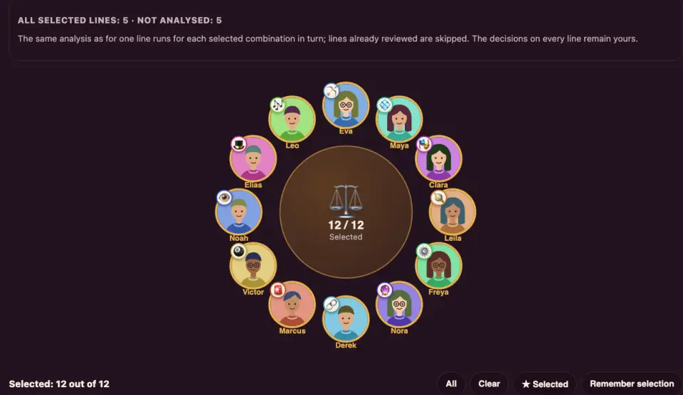
Selection of the twelve jurors around the Court emblem — The jury: twelve personas, each with its own mathematical strategy

The order of a case

Proposal. A juror or a model scans every possible single swap of the row and proposes at most one replacement — or proposes to keep the row.
Defence. Counsel take a position on each proposal: support, objection or protest. A counsel never proposes or applies a number.
Verdict. The Supreme Judge accepts the proposal, offers an alternative or keeps the number, using the structural field of past draws.
Decision. Only you change numbers: accept a proposal, follow the defence, accept the Judge, keep the original or revert. Each decision is stored with its author.

From a model to a per-number preference

Every model is reduced to a relative preference $\operatorname{rel}(n)$ for each number, where 1 means "the model's average", together with a standard error. Models defined by an explicit weight vector are exact; the others are measured by running them:

\operatorname{rel}(n) = \frac{w_n}{\frac{1}{N}\sum_m w_m}, \qquad \operatorname{se}(n) = 0

Exact relative preference of Hot numbers, Markov, Gauss, Bayes, Gap analysis, Quantum collapse, Quantum-astral and the Structural field.

\hat p_n = \frac{1}{R}\sum_{r=1}^{R} \bigl[\,n \in X_r\,\bigr], \quad \operatorname{rel}(n) = \frac{\hat p_n}{k/N}, \quad \operatorname{se}(n) = \frac{\sqrt{\hat p_n (1 - \hat p_n)/R}}{k/N}

Monte-Carlo preference of procedural models: X₁ … X_R are R = 600 seeded rows of the model (120 for the physical model). Consensus instead averages three runs (see its card).

The nineteen models

The Court uses the sixteen generator methods of section 2 plus three Court models. Four of them use no history and are registered as having no number preference (Segment coverage, Pure random, Physical model, Chaos); in practice Segment coverage favours the numbers of short segments when $k$ does not divide $N$ , and Chaos favours the edges of the range, as their cards show. Two models are composites (Consensus and Structural field).

Model	Type	Basis
Hot numbers	weights	$c_n + 0.05$
Combined	sampled	hot / middle / cold thirds
Segment coverage	sampled, no history	one number per segment
Pure random	sampled, uniform	Fisher–Yates shuffle
Markov chains	weights	smoothed transitions from the last draw
Gauss · CLT	weights	Gaussian around $\mu/k$
Interval model Δ	sampled	bootstrap of gaps
Bayes · Dirichlet	weights	$c_n + 3$
Gap analysis	weights	$(\operatorname{gap}/\bar g)^{1.6} + 0.15$
Physical model	sampled, no history	2D disc simulation
Chaos	sampled, no history	logistic map, edge-biased
Quantum collapse	weights, experimental	$e^{-1.15 c_n/\bar c} + 0.02$
System of paradoxes	sampled, experimental	five archetypes
Quantum-astral	weights, experimental	Moon sign and illumination
Wheel matrix	sampled	pair-coverage design
World hot	sampled	cross-lottery kernel profile
World combined	sampled	cross-lottery kernel profile
Consensus of models	ensemble	14 member models
Structural field	composite	six descriptive components

Structural field

Server

The field is the Supreme Judge's measure: a hand-weighted composite of six descriptive components. Frequencies, connectivity and pair coverage are divided by their maximum over all numbers; recency and typicality already lie in $[0,1]$ .

F(n) = 100\,\bigl(0.25\,A_n + 0.15\,S_n + 0.15\,G_n + 0.20\,L_n + 0.15\,T_n + 0.10\,(1 - P_n)\bigr)

Structural field score of number n, from 0 to 100.

Advanced details

where

$A_n,\ S_n$: frequency in the whole window and in the last $\max(3, \min(10, D))$ draws
$G_n$: recency, $\min(\operatorname{gap}_n/\bar g, 2)/2$
$L_n$: sum of pair lifts $\ell_{nm} = \dfrac{O_{nm}}{(c_n/D)(c_m/D)\,D}$ over all partners $m$ , with $O_{nm}$ the number of draws containing both
$T_n$: average structural typicality of the draws containing $n$ : $1 - 0.6 \cdot 2\,|e - \tfrac12| - 0.4 \min(|z_S|, 2)/2$ , with $e$ the share of even numbers and $z_S$ the standardised sum
$P_n$: pair coverage, the total number of pair observations involving $n$

Consensus of models

Server

Fourteen member models in twelve families each produce 10 rows; a number scores by how many models and families chose it, how often, and how evenly:

C(n) = 100\Bigl(0.40\,\frac{M_n}{14} + 0.25\,\frac{F_n}{12} + 0.20\,\frac{f_n}{\max_m f_m} + 0.15\,\min(\operatorname{stab}_n, 1)\Bigr)

Consensus score; the Court averages three independent runs and uses their spread as the standard error.

Advanced details

where

$M_n,\ F_n$: number of member models and of model families whose rows contain $n$
$f_n$: total number of rows containing $n$
$\operatorname{stab}_n$: mean number of appearances per member model that chose $n$ , divided by 10

Quantum-astral model

ServerExperimental

An entertainment model that weights numbers by the Moon on the target draw date, plus a small share of the structural field:

w_n = 1 + \bigl[\,n \bmod 12 = \sigma\,\bigr]\Bigl(0.10 + 0.20\,\frac{I}{100}\Bigr) + 0.15\,\frac{F(n)}{100}

Quantum-astral weight; σ ∈ {0,…,11} is the zodiac sign of the Moon's ecliptic longitude on the target draw date, I the illumination in percent.

Advanced details

I = 100 \cdot \frac{1 - \cos(2\pi A / P)}{2}, \qquad P = 29.530588853\ \mathrm{d}

Moon illumination in percent from the age A of the synodic month of length P (days).

How a model reviews a row

For each possible swap $a \to b$ — number $a$ leaves the row, number $b$ enters — the model computes the gain and its noise. A gain counts only if it is statistically clear; a loss always counts.

\delta = \operatorname{rel}(b) - \operatorname{rel}(a), \qquad z = \frac{\delta}{\operatorname{SE}_\delta}, \qquad \operatorname{effect} = \begin{cases} \delta & \operatorname{SE}_\delta = 0 \ \vee\ z \ge z^{*} \\ \min(\delta, 0) & \operatorname{SE}_\delta > 0 \ \wedge\ z < z^{*} \end{cases}

Model review. Exact weight models have SE = 0, so their gains always count; the swap qualifies when effect ≥ 0.10.

\operatorname{SE}_\delta = \frac{1}{k/N}\sqrt{\frac{2\,\bar p\,(1 - \bar p)}{R}}, \qquad \bar p = \max\!\Bigl(\frac{\operatorname{rel}(a) + \operatorname{rel}(b)}{2}\,\frac{k}{N},\ \frac{1}{2R}\Bigr)

Standard error of a swap for a sampled model: the pooled proportion under the hypothesis that a and b are equally likely. For Consensus SE_δ = √(se(a)² + se(b)²) over its three runs; exact weight models have SE_δ = 0.

z^{*} = \Phi^{-1}\!\Bigl(1 - \frac{1 - \Phi(1.5)}{k(N-k)}\Bigr)

Bonferroni-corrected threshold over all k(N−k) possible swaps; Eurojackpot: 3.43.

Base $z$	Eurojackpot, 225 swaps	Lotto 7/34, 189 swaps
0.5	2.995	2.942
1.0	3.193	3.142
1.5	3.434	3.387
2.0	3.716	3.672
3.0	4.378	4.340

The twelve jurors

Each juror has one strategy, its own sources (models or history signals), a minimum effect and a significance level. A juror's verdict on a row is either "keep" or exactly one replacement; jurors do not object or protest — that is the role of the defence.

\operatorname{score}(n) = \sum_m \omega_m \operatorname{rel}_m(n), \qquad \Delta = \lambda\,\bigl(\operatorname{score}(b) - \operatorname{score}(a)\bigr)

Numeric gain of a swap from the juror's weighted sources; λ = D/(D+40) for Eva Lind, otherwise 1.

E = \begin{cases} \Delta & \operatorname{SE}_\Delta = 0 \ \vee\ z \ge z^{*}(z_{\min}) \\ \min(\Delta, 0) & \operatorname{SE}_\Delta > 0 \ \wedge\ z < z^{*}(z_{\min}) \end{cases} \ +\ \omega_S \cdot 0.25 \sum_c \Delta \ell_c \ +\ \omega_C\,\Delta \Gamma, \qquad E \ge E_{\min} \ \Rightarrow\ a \to b

Effective value of a swap. The best qualifying swap wins (ties: smaller new number, then earlier position); with none, the juror keeps the row.

where

$\omega_m$: weight of source $m$ in the juror's definition
$z$: $\Delta / \operatorname{SE}_\Delta$ , with $\operatorname{SE}_\Delta = \lambda\sqrt{\sum_m (\omega_m \operatorname{SE}_m)^2}$
$z^{*}(z_{\min})$: the juror's significance level corrected for $k(N-k)$ swaps, as in the table above
$\Delta \ell_c$: change of the log-likelihood of structural component $c$ (nats)
$\Delta \Gamma$: change of the ticket coverage score

Signals computed from history

Three jurors use signals read directly from the draws rather than from a generator. With $p = k/N$ :

\operatorname{rel}(x) = \frac{c_x}{Dp}, \qquad \operatorname{SE}_{ab} = \sqrt{\frac{2(N-k)}{(N-1)\,p\,D}}

Frequency test. Under fair draws Var(c_a − c_b) = 2Dp(1−p)·N/(N−1) because numbers in one draw are negatively correlated; dividing by the expected count Dp gives SE_ab.

\operatorname{rel}(x) = \max\!\Bigl(0,\ \bar f_x - \frac{\operatorname{sd}(f_x)}{\sqrt K}\Bigr), \qquad f_{x,w} = \frac{c_{x,w}}{s\,p}, \qquad K = \min\!\bigl(4, \lfloor D/5 \rfloor\bigr)

Replication. Frequency in K disjoint windows of s = ⌊D/K⌋ draws; the advantage must survive a one-standard-error penalty.

\operatorname{raw}(x) = 1 + \left|\frac{c_x - Dp}{\sqrt{Dp(1-p)}}\right|, \qquad \operatorname{rel} = \frac{\operatorname{raw}}{\overline{\operatorname{raw}}}, \qquad \operatorname{SE} = \frac{\sqrt{1 - 2/\pi}}{\overline{\operatorname{raw}}}

Anomaly. Absolute deviation from the expected count; √(1−2/π) is the standard deviation of |Z| for a standard normal Z.

Structure and coverage

Structural components compare a row with the profile of past draws: parity, low/high, clusters and gaps are categorical with Laplace smoothing; sum and spread are Gaussian.

\ell_1 = \ln\frac{n_j + 1}{D + J}, \qquad \ell_2 = -\frac12\Bigl(\frac{x - \mu}{\sigma}\Bigr)^2, \qquad \ell_3 = \frac{1}{k-1}\sum_{i} \ln\frac{n_{\Delta_i} + 1}{n_\Delta + N}

Log-likelihoods: ℓ₁ categorical (parity, low/high, clusters; J categories, n_j past draws in category j), ℓ₂ Gaussian (sum, spread), ℓ₃ gaps between neighbouring numbers.

\Gamma(R) = -\frac{\bigl|\tbinom{R}{2} \cap \mathcal P'\bigr|}{\binom{k}{2}} + 0.5\,\frac{\bigl|\{\lfloor (n-1)/10 \rfloor : n \in R\}\bigr|}{k}

Ticket coverage: 𝒫′ is the set of pairs of the other rows of the ticket; the second term counts the decades of the number field that the row touches.

Eva Lind · Sharpshooter

Strategy: long-run frequency with Bayesian shrinkage. Sources: Bayes 0.8 + Hot numbers 0.2; $\lambda = D/(D+40)$ ; $E_{\min} = 0.12$ ; no significance test (exact weights).

Rule: the best swap is always the least frequent number of the row → the most frequent number outside it; it qualifies when $\Delta \ge 0.12$ .

Advanced details

Maya Chen · Shape Architect

Strategy: the shape of the row. Sources: Gauss 0.5 + Combined 0.5; structure weight 2 on parity, low/high, sum, spread and clusters; $z_{\min} = 1$ (Eurojackpot $z^{*} = 3.19$ ); $E_{\min} = 0.12$ .

Rule: the structure term always counts, so a swap that brings the row closer to the typical shape of past draws can qualify on structure alone.

Advanced details

Clara Moretti · Anomaly Hunter

Strategy: anomalies in either direction. Source: the anomaly signal; gaps structure 0.4 counted only for a significant swap; $z_{\min} = 1.5$ (Eurojackpot $z^{*} = 3.43$ ); $E_{\min} = 0.10$ .

z = \frac{|z_b| - |z_a|}{\sqrt 2 \cdot 0.60281}

For the anomaly signal the mean cancels: only the difference of absolute deviations matters.

Advanced details

Leila Haddad · Global Observer

Strategy: the world profile. Sources: World hot 0.5 + World combined 0.5; $z_{\min} = 1.5$ ; $E_{\min} = 0.12$ ; needs data of the other lotteries.

Advanced details

Freya Olsen · Coverage Engineer

Strategy: ticket coverage with no number preference. No sources; coverage weight 2; $E_{\min} = 0.20$ .

Advanced details

Nora Blake · Clairvoyant

Experimental

Strategy: the entertainment astro system for the draw date. Source: Quantum-astral; $E_{\min} = 0.05$ ; needs a target draw date.

Advanced details

Derek Cole · Chain Master

Strategy: transitions from the latest draw. Source: Markov chains; gaps structure 0.4, always counted; $E_{\min} = 0.12$ . Because the Markov weights sum to one, $\operatorname{rel}(n) = N\,w_n$ .

Advanced details

Marcus Reed · Alarm Signal

Strategy: the longest absence. Sources: Gap analysis 0.8 + Hot numbers 0.2; $E_{\min} = 0.06$ ; no significance test.

Advanced details

Victor Moreau · Drum Physicist

Strategy: a physical bias of the drum would repeat in every period. Source: replication; $z_{\min} = 2$ (Eurojackpot $z^{*} = 3.72$ ); $E_{\min} = 0.15$ .

\operatorname{SE}_{ab} = \max\!\Bigl(\frac{\operatorname{sd}_w(f_{b,w} - f_{a,w})}{\sqrt K},\ \sqrt{\frac{2(N-k)}{(N-1)\,p\,K s}}\Bigr)

The noise floor prevents four lucky windows from looking significant.

Advanced details

Noah Bennett · Vigilant Skeptic

Strategy: reject pure chance at the strictest level. Source: frequency test; $z_{\min} = 3$ (Eurojackpot $z^{*} = 4.38$ ); $E_{\min} = 0.15$ .

z = \frac{c_b - c_a}{\sqrt{2(N-k)\,Dp/(N-1)}}

Closed form of Noah's test statistic.

Advanced details

Elias Berg · Contrarian Magician

Experimental

Strategy: against the crowd — rarer numbers. Sources: Quantum collapse 0.85 + System of paradoxes 0.15; $z_{\min} = 0.5$ (Eurojackpot $z^{*} = 3.00$ ); $E_{\min} = 0.08$ .

Advanced details

Leo Fischer · Consensus Conductor

Strategy: the stability of the model consensus. Source: Consensus (three independent runs); $z_{\min} = 2$ (Eurojackpot $z^{*} = 3.72$ ); $E_{\min} = 0.10$ .

Advanced details

Jury generation

When the jury generates a row instead of reviewing one, each juror draws 40 candidate rows from its own weights $\max(0.02, \operatorname{score}(n))$ and keeps the best by

\operatorname{rowScore}(R) = \frac{1}{k}\sum_{n \in R} \operatorname{score}(n) + \omega_S \cdot 0.25 \sum_c \ell_c(R) + \omega_C \operatorname{cov}(R)

A juror's ballot. The jury row takes the k numbers with the most ballots; ties go to the higher normalised support, then to the smaller number.

The six defence counsel

Counsel evaluate a proposed swap $n_c \to n_p$ — the current number and the proposed one, drawn $x_c$ and $x_p$ times in $D$ draws — with their own signals. Positive values favour the proposal:

Signal	Definition
frequency	$z = \dfrac{(x_p - x_c)/D}{\sqrt{2\bar p(1-\bar p)/D}},\ \bar p = \dfrac{x_c + x_p}{2D}$
posterior	$z = \Phi^{-1}\bigl(P(\theta_p > \theta_c)\bigr),\ \theta \sim \operatorname{Beta}(1 + x, 1 + D - x)$
Bayes, field, astro	$z = \dfrac{\operatorname{rel}(p) - \operatorname{rel}(c)}{\sqrt 2\,\operatorname{sd}(\operatorname{rel})}$
structure	$z = \operatorname{sign}(\Delta\ell)\sqrt{2\|\Delta\ell\|}$
stability	$z = (W - L)/\sqrt{6}$ over six consecutive periods

The posterior probability is computed exactly, without a normal approximation:

P(\theta_B > \theta_A) = \sum_{i=0}^{a_B - 1} \frac{\mathrm B(a_A + i,\ b_A + b_B)}{(b_B + i)\,\mathrm B(1 + i,\ b_B)\,\mathrm B(a_A, b_A)}

Closed form for Beta posteriors with integer parameter; the Beta function uses a Lanczos log-Gamma.

Decision rule for the replacement, with $\bar z$ the weighted mean of the counsel's signals:

\psi = \begin{cases} \mathsf S & \bar z \ge z_{\mathrm{sup}} \ \wedge\ \chi = 1 \\ \mathsf P & \bar z \le -z_{\mathrm{prot}} \ \wedge\ \chi = 1 \\ \mathsf O & \bar z \in (-z_{\mathrm{prot}},\ z_{\mathrm{sup}}) \ \vee\ \chi = 0 \end{cases}

Position ψ of a counsel: S support, P protest, O objection. χ = 1 when the counsel's checks pass: for support — unanimity of signals, agreement of a second signal and the structural veto; for protest — unanimity and agreement only.

Thomas Keller · Assigned counsel

FREE

Signals: frequency + Bayes + structural field, all must agree; support at 1, protest at −1; needs 20 draws, and from 5 to 19 draws works in a limited mode with Bayes + posterior.

Advanced details

Elena Rossi · Statistical counsel

Signal: frequency, corrected for multiple comparisons; structural veto at −1; support and protest at 1.96; at least 30 draws.

Advanced details

Amelia Grant · Against false confidence

Signal: posterior probability of superiority; support at $P \ge 0.90$ ( $z = 1.2816$ ), protest at $P \le 0.20$ ( $z = -0.8416$ ); at least 10 draws.

Advanced details

$D$	$x_c$	$x_p$	$P(\theta_p > \theta_c)$	Position
30	1	7	0.987	support
30	4	3	0.354	objection
30	5	2	0.128	protest
100	6	16	0.987	support

Julien Morel · Structure counsel

Signal: total change of the six structural log-likelihoods; support at 0.6325 ( $\Delta\ell \ge 0.2$ nats), protest at 0.8944 ( $\Delta\ell \le -0.4$ ); at least 20 draws.

Advanced details

Ingrid Falk · Stability over time

Signal: wins minus losses of the proposed number over six consecutive periods; must agree with the overall frequency; threshold 1.5, so at least $W - L \ge 4$ ; at least 30 draws.

Advanced details

Adrian Vega · Entertainment astrology

Experimental

Signal: the Quantum-astral weights for the target draw date; support and protest at 0.5.

Advanced details

The Supreme Judge

The Judge rules on a disputed number using the structural field $F$ , normalised to its maximum: $\phi(n) = F(n)/\max F$ . A number is weak if it lies in the lowest 35% of the field.

\theta = \phi_{(\lfloor 0.35 N \rfloor + 1)}, \qquad m = 0.08 \cdot \bigl[\, n_{\mathsf P} > \tfrac12\, n_{\mathrm{counsel}} \,\bigr]

θ is an order statistic of the field values sorted in ascending order; the current number is weak when φ(n_c) < θ. The margin m applies when more than half of the counsel with a position protest.

V = \begin{cases} n_c & \phi(n_c) \ge \theta \\ n_p & \phi(n_p) > \phi(n_c) + m \ \wedge\ \phi(n_p) \ge \theta \\ a^{*} & \phi(a^{*}) > \phi(n_c) + m \\ n_c & \phi(a^{*}) \le \phi(n_c) + m \end{cases}

The verdict V is the number that the Judge keeps in the position; the first matching line applies. a* is the number with the highest field outside the row and other than the proposal.

Supreme Judge analysis and recommendation

For whole rows the Judge reports a row score and suggests replacing up to $\lfloor k/2 \rfloor$ of the weakest numbers below $\theta$ by the strongest numbers outside the row. You choose which swaps to apply. With no rows, the Judge recommends: uniform random drafts are improved in the same way and returned with their provenance.

\operatorname{RowScore}(R) = \frac{100}{k}\sum_{n \in R} \phi(n)

Row score of the Supreme Judge analysis.

Decisions, batches and history

Decisions: accept the proposal, accept the defence, accept the Judge, keep the original, revert. Numbers change only when you accept a proposal, accept a Judge verdict that replaces the number, or revert; each change is a transformation in the provenance record.
Bulk decisions: at most one replacement per number. "Accept all majority replacements" applies only options chosen by more than half of the selected jurors; "Apply all proposals" takes, for each number, the majority option or else the one with the most votes, and skips ties.
Batches: a review of up to 50 rows by the same line-up of personas counts as one attempt; rows already analysed are skipped and an interrupted batch resumes with the same plan.
History: event types are jury review, model review, proposal, defence review, Judge review, decision and transformation; the log keeps up to 200 events and never drops a transformation or the latest reviews.

Holding the Court to account

Every claim is written to the prediction ledger before its draw and scored afterwards against chance. For claims about $n_i$ numbers with base chance $p = k/N$ :

\mathbb E[H] = \sum_i n_i\,p, \qquad \operatorname{Var}[H] = \sum_i n_i\,p(1-p), \qquad \operatorname{lift} = \frac{H}{\mathbb E[H]}, \qquad z = \frac{H - \mathbb E[H]}{\sqrt{\operatorname{Var}[H]}}

H is the number of hits. A source is ranked only with at least 30 numbers over at least 3 draws.

4. The 3D drum: physics engine

The 3D draw is a real-time rigid-body simulation: balls are bodies with mass, inertia, friction and restitution, pushed by gravity, a stirring rotor and an air field, and the drawn ball is the one that physically falls through the outlet. It is a credible physical model of a drum, not a recording of a real machine.

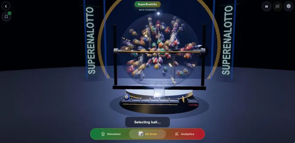
SuperEnalotto drum with 90 balls being mixed while a ball is selected — 90 SuperEnalotto balls in the simulated chamber

Engine and coordinates

Physics runs in Rapier 3D (version 0.14, WebAssembly); rendering uses Three.js (r169). The world is right-handed with $+y$ up and the origin at the centre of the chamber; the rotor axis is the horizontal $x$ axis and $+z$ points towards the viewer.

Chamber: a sphere of radius $R = 3.0$ units, built as a triangle mesh with inward normals and a circular outlet at the bottom (half-angle $\arcsin(0.34/3) \approx 6.5^\circ$ ).
Balls: spheres of radius $r = 0.2$ and density 1; one ball per number, from 5 to 90 balls.
Rotor: a kinematic shaft with six arms whose capsule paddles are sized to stop 0.14 units from the glass in their plane of rotation, plus a smaller three-arm rotor whose direction alternates between mix phases.
Gate: a cylindrical plug in the outlet, removed when a ball may leave.

m = \tfrac43 \pi r^3 \rho = 0.03351, \qquad I = \tfrac25 m r^2 = 5.36 \times 10^{-4}, \qquad m\,|g| = 1.005

Mass, moment of inertia and weight of a ball in model units.

Scale and Froude similarity

One model unit is 10 cm: a 40 mm ball is 0.4 units and the chamber is a 600 mm sphere. Gravity is reduced to $30$ units/s² instead of the real $98.1$ . Motion dominated by gravity and inertia looks the same when the Froude number is the same, so the simulation corresponds to a real-size machine with a slower clock:

\mathrm{Fr} = \frac{v^2}{g L}, \qquad \gamma = \frac{g'}{g} = \frac{30}{98.1} = 0.306, \qquad \frac{t'}{t} = \frac{1}{\sqrt\gamma} \approx 1.81

Primed quantities belong to the model. Equal Froude number at equal length: velocities scale with √γ and times with 1/√γ.

Forces

Every ball obeys Newton's second law with the forces that the code actually applies:

m\,\frac{d^2 \mathbf x}{dt^2} = m\,\mathbf g + \mathbf F_D + \mathbf F_W + \mathbf F_S + \mathbf F_C, \qquad I\,\frac{d\boldsymbol\omega}{dt} = \boldsymbol\tau_W + \boldsymbol\tau_C

F_D air drag, F_W analytic wall, F_S suction at the outlet, F_C contacts with balls, rotor and gate (computed by Rapier); τ the corresponding torques. Rapier also applies small linear and angular damping, and speeds are capped at 22 units/s and 105 rad/s as a safety net.

Air field and quadratic drag

The blower is modelled as a prescribed air-velocity field $\mathbf u(\mathbf x, t)$ ; each ball feels quadratic drag towards the local air velocity. The drag constant is fixed by a terminal speed of 48 units/s:

\mathbf F_D = m\,k_d\,\lVert \mathbf u - \mathbf v \rVert\,(\mathbf u - \mathbf v), \qquad k_d = \frac{|g|}{v_t^2} = \frac{30}{48^2} = 0.01302

In still air a falling ball reaches v_t = √(g/k_d) = 48 units/s, about 8.7 m/s at real scale.

u_y^{\uparrow} = J \Bigl(1 - \frac{\rho_h^2}{R^2}\Bigr)\, \operatorname{clamp}\!\Bigl(\frac{6 - y}{6 + R},\, 0,\, 1\Bigr), \qquad J = 102

Central updraft: strongest on the axis near the bottom (102 at y = −3, 68 at the centre, 34 at the top); ρ_h is the horizontal distance from the axis.

Swirl: a horizontal rotation of 11 units/s about the vertical axis.
Inward flow: beyond 60% of the radius, up to $50\,(|\mathbf x| - 1.8)/1.2$ towards the centre, so balls keep cycling instead of hugging the glass.
Turbulence: smooth three-dimensional value noise of amplitude 58 that drifts in time; it is a fixed deterministic function, not a random number generator.
Anti-stall gusts: a ball that stays too long at the bottom, at the top, at the wall or almost motionless gets a local gust added to the air velocity, still acting through drag.

Analytic spherical wall

On top of the mesh, the glass is enforced as an exact sphere at the velocity level, which prevents tunnelling and gives correct rolling. With outward normal $\hat{\mathbf n}$ , outward speed $v_n$ and penetration $\xi = |\mathbf x| - (R - r - 0.06)$ :

v^{*} = \begin{cases} -\min\!\bigl(2,\ 0.25\,\xi/\Delta t\bigr) & \xi > 0 \\ -\xi/\Delta t & \xi \le 0 \end{cases}, \qquad e = \begin{cases} \tfrac12 (e_b + 0.28) & v_n > 0.6 \\ 0 & v_n \le 0.6 \end{cases}

Speculative contact allowance v* and restitution e (e_b is the ball's restitution; zero below the slop speed so a resting ball cannot buzz).

\Delta v_n = v_n - \min(v^{*},\, -e\,v_n), \qquad \mathbf F_n = -\frac{m\,\Delta v_n}{\Delta t}\,\hat{\mathbf n}

Normal response, applied only if v_n > v*.

j_t = \min\!\Bigl(\mu\, m\,\Delta v_n,\ \tfrac27 m\,\lVert \mathbf s \rVert\Bigr), \qquad \mathbf F_t = -\frac{j_t}{\Delta t}\,\hat{\mathbf s}, \qquad \boldsymbol\tau = (-r\hat{\mathbf n}) \times \mathbf F_t

Coulomb friction at the contact point; s is the tangential slip velocity v + ω × (−r n̂), μ = ½(μ_b + 0.35) with μ_b the ball's friction.

Contacts between bodies

Ball–ball, ball–rotor and ball–gate contacts are solved by Rapier's constraint solver with continuous collision detection on the balls. Coefficients are combined by averaging:

Pair	Friction	Restitution
ball – ball	0.16	0.55
ball – glass	0.255	0.415
ball – paddle	0.19	0.525
ball – arm or shaft	0.17	0.35
ball – gate	0.23	0.375

Damping is small during the draw (linear 0.05, angular 0.035) and strong while balls settle (2.4). There is no rolling resistance parameter: rolling slows only through damping and contact friction.

Time stepping and integration

The simulation advances in fixed steps independent of the screen refresh rate; each frame runs as many fixed steps as real time requires, at most five:

A \leftarrow \min\bigl(A + \Delta t_f,\ 5\,\Delta t\bigr), \qquad n = \bigl\lfloor A / \Delta t \bigr\rfloor, \qquad A \leftarrow A - n\,\Delta t, \qquad \Delta t = \tfrac{1}{60}\ \mathrm{s}

Fixed-step accumulator: a frame of duration Δt_f runs n fixed steps (at most 5); each step is split into 2 Rapier sub-steps of h = 1/120 s with 6 solver iterations.

Within a sub-step the engine updates velocities from forces and then positions from the new velocities — the semi-implicit (symplectic) Euler scheme used by impulse-based engines, shown here as the general principle:

\mathbf v_{t+h} = \mathbf v_t + h\,M^{-1}\bigl(\mathbf F + \mathbf F_{\mathrm c}\bigr), \qquad \mathbf x_{t+h} = \mathbf x_t + h\,\mathbf v_{t+h}

General form: F are the applied forces, F_c the constraint (contact) forces found by Rapier's iterative solver.

The application's own forces (air, wall, suction) are computed once per step from the state at its start and held over both sub-steps. The rotor is kinematic and is re-targeted every sub-step:

\omega \leftarrow \omega + (\omega^{*} - \omega)\bigl(1 - e^{-4h}\bigr), \qquad \theta \leftarrow \theta + \omega\,h

Exponential approach of the rotor speed to its target; the mix cycles through 2.4, 2.9, 2.1 and 2.7 rad/s.

How a ball is selected

After 1 s of start-up and 2.6 s of mixing the gate opens. While the outlet is open the updraft above it collapses smoothly, the central jet is reduced to 62% and a suction of about 2.2 ball weights (about 4 after 5 s) pulls balls near the outlet:

\mathbf F_S = \beta\,(-1.2\,x,\ -2.2,\ -1.2\,z), \qquad \beta = \begin{cases} 1 & t_c \le 5\ \mathrm{s} \\ 1.8 & t_c > 5\ \mathrm{s} \end{cases}

Suction near the outlet (y < −1.6 and horizontal distance < 0.6); t_c is the time since the gate opened.

The drawn ball is the first one whose centre falls below $y = -3.18$ ; if several do in the same step, the lowest. No random number is consulted at that moment. The random numbers of a draw are the initial placement of the balls and a small initial velocity and spin, taken from the Web Crypto API (again when a separate bonus pool is loaded). The ball then travels along the exit path to the rack; that motion is scripted, not simulated.

Rendering versus simulation versus randomness

Simulation: fixed 1/60 s steps; quality presets (ultra, high, medium, low) change shadows, bloom, resolution and mesh detail only, never the physics.
Rendering: each frame shows the last completed step; there is no interpolation between steps.
Randomness: the forces are deterministic; the outcome depends on the initial placement and, from the second ball on, also on how long the reveal of the previous ball takes on the device, so a draw cannot be replayed exactly.

5. Statistics of real draws

The analytics screens describe historical draws. They answer "what happened" and "is this consistent with a fair lottery", never "what will happen".

Frequencies, hot and cold

For each number the app counts appearances in the window and shows them next to the expected count of a fair lottery; the standard deviation is given here for reference:

\mathbb E[c_n] = \frac{kD}{N}, \qquad \operatorname{sd}(c_n) = \sqrt{D\,\frac{k}{N}\Bigl(1 - \frac{k}{N}\Bigr)}

Expected count (shown in the app) and its standard deviation (reference) for one number over D independent draws.

Hot and cold: the five most and least frequent numbers, each with its expected count (at least 5 draws are required).
Frequency bars: red when a number's share exceeds 1.3 times the expected share, blue below 0.7 times.
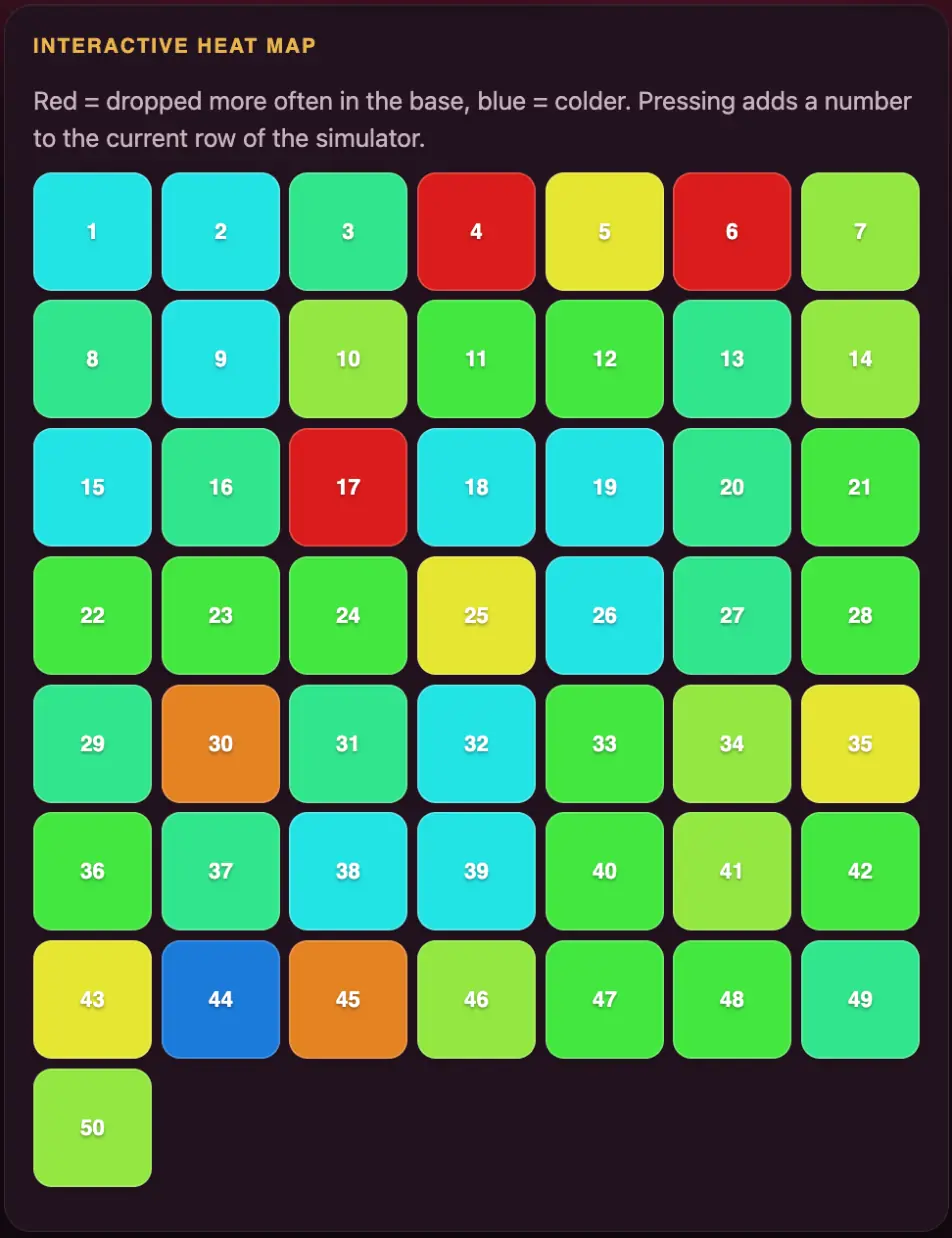
Heat map: colour by min–max normalisation $s_n = (c_n - \min c)/\max(1, \max c - \min c)$ .

Eurojackpot heat map of the 50 main numbers coloured from blue to red — Heat map: colour shows past frequency only

Fairness test: χ² with a correction

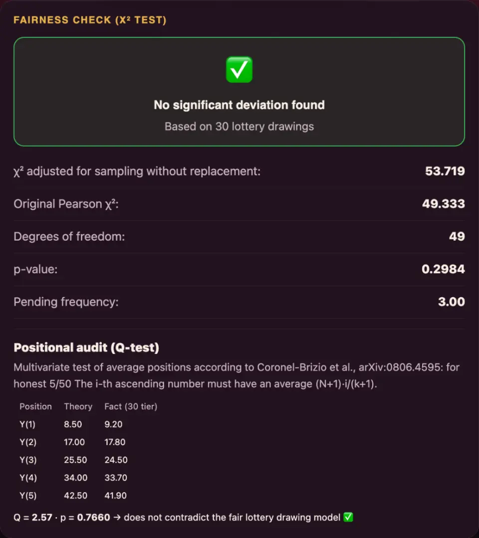
The χ² test checks whether the counts are consistent with equal probabilities. In one draw the $k$ numbers are taken without replacement, which makes counts negatively correlated; the plain multinomial statistic is then too small, and the app corrects it:

\chi^2_P = \sum_{n=1}^{N} \frac{(c_n - e)^2}{e}, \quad e = \frac{kD}{N}, \qquad \chi^2 = \chi^2_P\,\frac{N-1}{N-k} \ \sim\ \chi^2_{N-1}

Pearson statistic with the without-replacement correction; at least 10 draws are required.

p = Q\Bigl(\frac{N-1}{2},\ \frac{\chi^2}{2}\Bigr) = \frac{\Gamma\bigl(\frac{N-1}{2}, \frac{\chi^2}{2}\bigr)}{\Gamma\bigl(\frac{N-1}{2}\bigr)}

Regularised upper incomplete gamma function, computed by series and continued fraction.

p-value	Verdict
$p > 0.05$	no significant deviation
$0.01 < p \le 0.05$	borderline deviation
$p \le 0.01$	statistically significant deviation

Positional Q-test

With at least 30 complete draws the app also tests the average of each sorted position (Coronel-Brizio et al., arXiv:0806.4595). The $i$ -th smallest of $k$ numbers drawn from $1..N$ has mean and covariance

\mu_i = \frac{(N+1)\,i}{k+1}, \qquad V_{ij} = \frac{i\,(k - j + 1)(N+1)(N-k)}{(k+1)^2 (k+2)}\ \ (i \le j), \qquad Q = m\,\boldsymbol\delta^{\mathsf T} V^{-1} \boldsymbol\delta \ \sim\ \chi^2_k

δ is the vector of differences between the observed position means and μ over m draws.

Pairs, comparisons and checks

Pairs: a 12 × 12 matrix of how often the 12 most frequent numbers appeared together (at least 10 draws). These are raw counts; for reference, the expected count of a given pair in fair draws is $D\,\frac{k(k-1)}{N(N-1)}$ .
Comparison of lotteries: jackpot odds, price, the cost of buying every combination.
Mathematics check: the app recomputes $\binom{N}{k}\binom{B}{b}$ and compares it with the stored constant, and checks the draws of the analysis window for range errors, wrong ball counts and duplicate dates.
Prize tiers: official payout tables per draw. The draw picture averages the last 60 real payout tables; only for a lottery with no payout data at all does it estimate winners from the tier probabilities of section 8 and an assumed sales volume, so those figures are illustrative.

Simulating a lifetime of play

The 50-year simulation uses the probability of at least one jackpot in $T$ independent tickets:

P_T = 1 - \Bigl(1 - \frac{1}{C}\Bigr)^{T}, \qquad T = 50 \cdot 52 \cdot d \cdot r

Probability of at least one jackpot in T tickets; C is the number of jackpot combinations, d draws per week, r rows per draw.

6. Calendar analysis

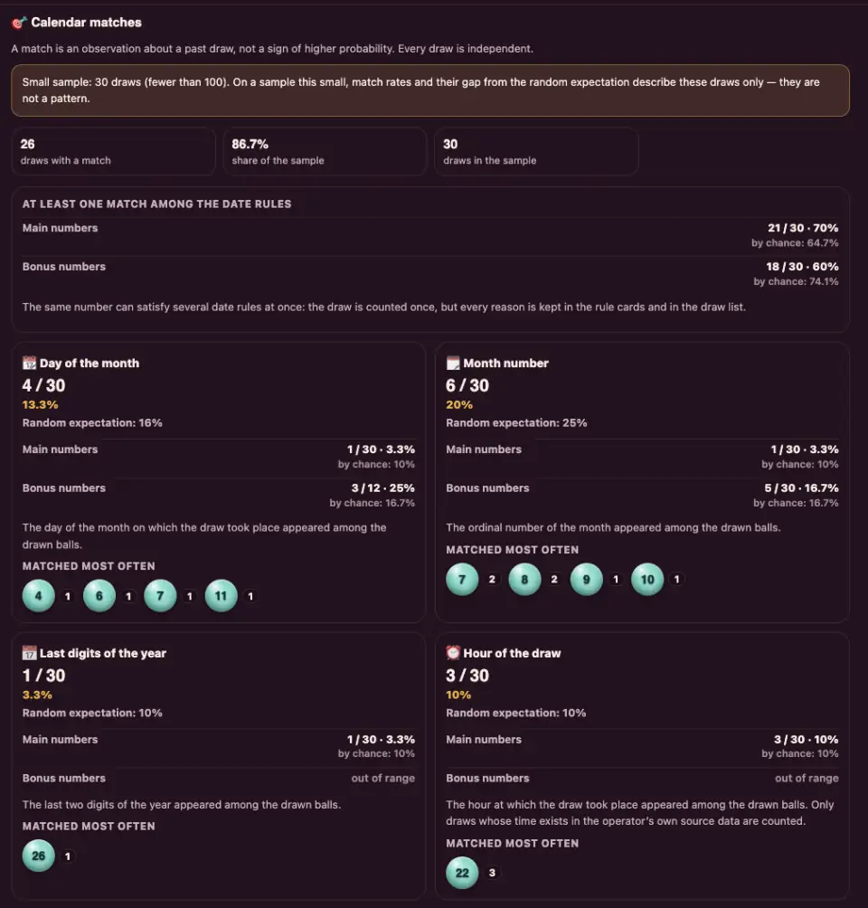
Calendar analysis looks for coincidences between draw dates and drawn numbers — for example the day of the month appearing among the balls — and compares each observed rate with the rate that pure chance would produce.

Selecting draws

Draws can be filtered by year, month, the same month across all years or a date range, and by rule era. Frequency lists (hot, cold, longest absent) use raw counts in the selection; a number that is impossible in every selected era is left out, and a selection that mixes eras is flagged with a warning, because a number valid only in the newer era looks falsely "cold". The date rules below are era-aware: a draw counts for a rule only if at least one candidate is a valid number of that draw's own rules.

\hat r = \frac{\bigl|\{\, t \in \mathcal E : C_t \cap X_t \ne \varnothing \,\}\bigr|}{|\mathcal E|}, \qquad \mathcal E = \bigl\{\, t : C_t \cap \Omega_t \ne \varnothing \,\bigr\}

Observed rate of a date rule: C_t are the candidate numbers of draw t, X_t its drawn numbers, Ω_t the valid numbers under its rules; ℰ are the eligible draws.

Ten date rules

Rule	Candidate numbers for a draw on DD.MM.YYYY
day	DD
month	MM
year	YYYY mod 100
hour	the hour of the draw, where the operator publishes it
year digits	the distinct digits of YYYY
year digit sum	sum of the digits of YYYY
two-digit year sum	sum of the digits of YYYY mod 100
day digit sum	sum of the digits of DD
date digit sum	sum of all digits of DD, MM and YYYY
digital root	the date digit sum reduced to one digit

A candidate equal to 0 is ignored, and a draw counts once for a rule even when several of its numbers match.

Random expectation

For a draw of $k$ numbers from $S$ possible values and a set of $m$ candidate numbers, the probability that no candidate is drawn is hypergeometric:

P_0 = \prod_{i=0}^{k-1} \frac{S - m - i}{S - i} = \frac{\binom{S-m}{k}}{\binom{S}{k}}, \qquad P_{\ge 1} = 1 - P_0

P₀: no candidate is drawn; P≥1: at least one is. Candidates outside the range of the draw's era are discarded.

\mathbb E[\hat r] = \frac{1}{|\mathcal E|}\sum_{t \in \mathcal E} P_{\ge 1}^{(t)}, \qquad P^{\cup} = 1 - \bigl(1 - P^{\mathrm M}\bigr)\bigl(1 - P^{\mathrm B}\bigr)

Expected match rate r̂ over the eligible draws ℰ, each with its own era; P^M and P^B for the main and bonus pools are combined as independent.

Calendar matches with observed rates next to the random expectation — Calendar matches compared with chance

Interpreting the rates

Pairs are listed from 30 draws and triples from 120 (only combinations seen at least twice, the ten most frequent); below 100 draws a small-sample warning is shown. With 100 draws a rate near 20% still has a 95% band of about $\pm 1.96\sqrt{0.2 \cdot 0.8/100} \approx \pm 7.8$ percentage points.

7. Historical archive and rule eras

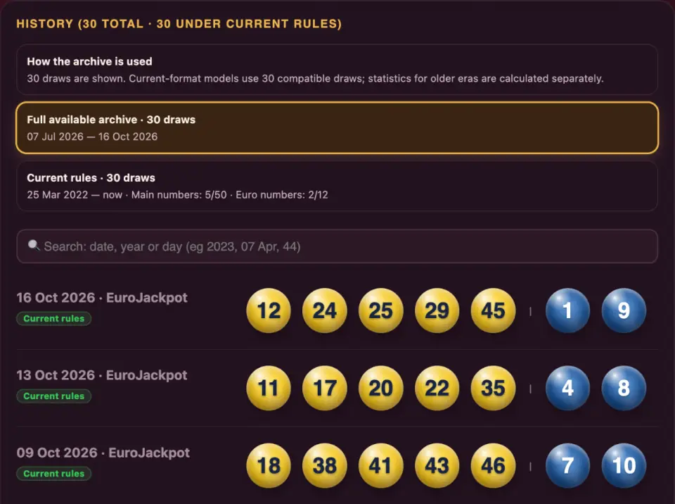
Lotteries change their rules. A draw is meaningful only together with the rules in force on its date, so every stored draw carries its rule version.

Rule eras

Lottery	Eras (main · bonus)
Lotto (Norway)	7/34 + 3 supplementary → 7/34 + 1 supplementary (from 21.03.2015)
Vikinglotto	6/48 + supplementary and lucky number → Viking number 1–8 (2017) → 1–5 (from 09.06.2021)
Eurojackpot	5/50 + 2/8 → 2/10 (2014) → 2/12 (from 25.03.2022)
Powerball	5/59 + 1/39 → 5/59 + 1/35 (2012) → 5/69 + 1/26 (from 07.10.2015)
Mega Millions	5/52 + 1/52 → 5/56 + 1/46 → 5/75 + 1/15 → 5/70 + 1/25 → 5/70 + 1/24 (from 08.04.2025)
EuroMillions	5/50 + 2/9 → 2/11 (2011) → 2/12 (from 27.09.2016)
SuperEnalotto	6/90 + Jolly since 1997; SuperStar is a separate drum and is excluded from the models
Lotto Max	7/49 → 7/50 (2019) → 7/52 (from 14.04.2026)
Powerball AU	5/45 + 1/45 → 6/40 + 1/20 (2013) → 7/35 + 1/20 (from 19.04.2018)

Compatibility rule

Models and analytics use only draws comparable with today's rules. Two eras are compared group by group:

(k, n_{\min}, n_{\max})_e = (k, n_{\min}, n_{\max})_{\mathrm{now}}, \qquad \mathcal B_e = \mathcal B_{\mathrm{now}}

Era e is comparable for main numbers when count and range agree (left), and for bonus numbers when every bonus group 𝓑 agrees (right). A draw with comparable main numbers but different bonus rules keeps its main numbers and drops its bonus numbers.

Eurojackpot history with the current-rules era card and draws marked with their rule version — The archive marks each draw with its rule era

8. Probability and limitations

Every official draw is an independent random experiment. No history, model, court or simulation changes the probability of any combination.

Jackpot probability

P_J = \frac{1}{\binom{N}{k}\binom{B}{b}}, \qquad \frac{1}{\binom{50}{5}\binom{12}{2}} = \frac{1}{2\,118\,760 \times 66} = \frac{1}{139\,838\,160}

Jackpot probability of one row under current rules (right: Eurojackpot); lotteries without a player bonus number use only the first factor.

Lottery	Rules	Jackpot odds
Lotto (Norway)	7/34	1 : 5 379 616
Vikinglotto	6/48 + 1/5	1 : 61 357 560
Eurojackpot	5/50 + 2/12	1 : 139 838 160
EuroMillions	5/50 + 2/12	1 : 139 838 160
Powerball	5/69 + 1/26	1 : 292 201 338
Mega Millions	5/70 + 1/24	1 : 290 472 336
SuperEnalotto	6/90	1 : 622 614 630
Lotto Max	7/52	1 : 133 784 560
Powerball AU	7/35 + 1/20	1 : 134 490 400

Every prize tier

Matching exactly $i$ of the $k$ main numbers and $j$ of the $b$ bonus numbers is a product of two hypergeometric probabilities:

P(i, j) = \frac{\binom{k}{i}\binom{N-k}{k-i}}{\binom{N}{k}} \cdot \frac{\binom{b}{j}\binom{B-b}{b-j}}{\binom{B}{b}}

For an extra ball drawn from the same drum (Lotto, SuperEnalotto, Lotto Max) the second factor is (k−i)/(N−k) for "+1".

Eurojackpot tier	Odds
5 + 2	1 : 139 838 160
5 + 1	1 : 6 991 908
5 + 0	1 : 3 107 515
4 + 2	1 : 621 503
4 + 1	1 : 31 075
3 + 2	1 : 14 125
4 + 0	1 : 13 811
2 + 2	1 : 985
3 + 1	1 : 706
3 + 0	1 : 314
1 + 2	1 : 188
2 + 1	1 : 49

Why no method can beat chance

If draws are independent and every combination is equally likely, the conditional probability of the next draw given any history is the same as without it, and the expected number of matched main numbers is the same for every row, however it was produced:

P\bigl(X_{t+1} = A \mid X_1, \dots, X_t\bigr) = P(X_{t+1} = A) = \binom{N}{k}^{-1}, \qquad \mathbb E[H] = k \cdot \frac{k}{N}

H is the number of matched main numbers of a row. Eurojackpot: 5 · 5/50 = 0.5 per row for every method.

Open Lotto Simulator